5 Genetic Diversity
➡️ This section includes four subpages: Diversity Parameter, Circos Plot, Genetic Distance, and AMOVA, allowing you to conduct various population diversity and differentiation analyses.
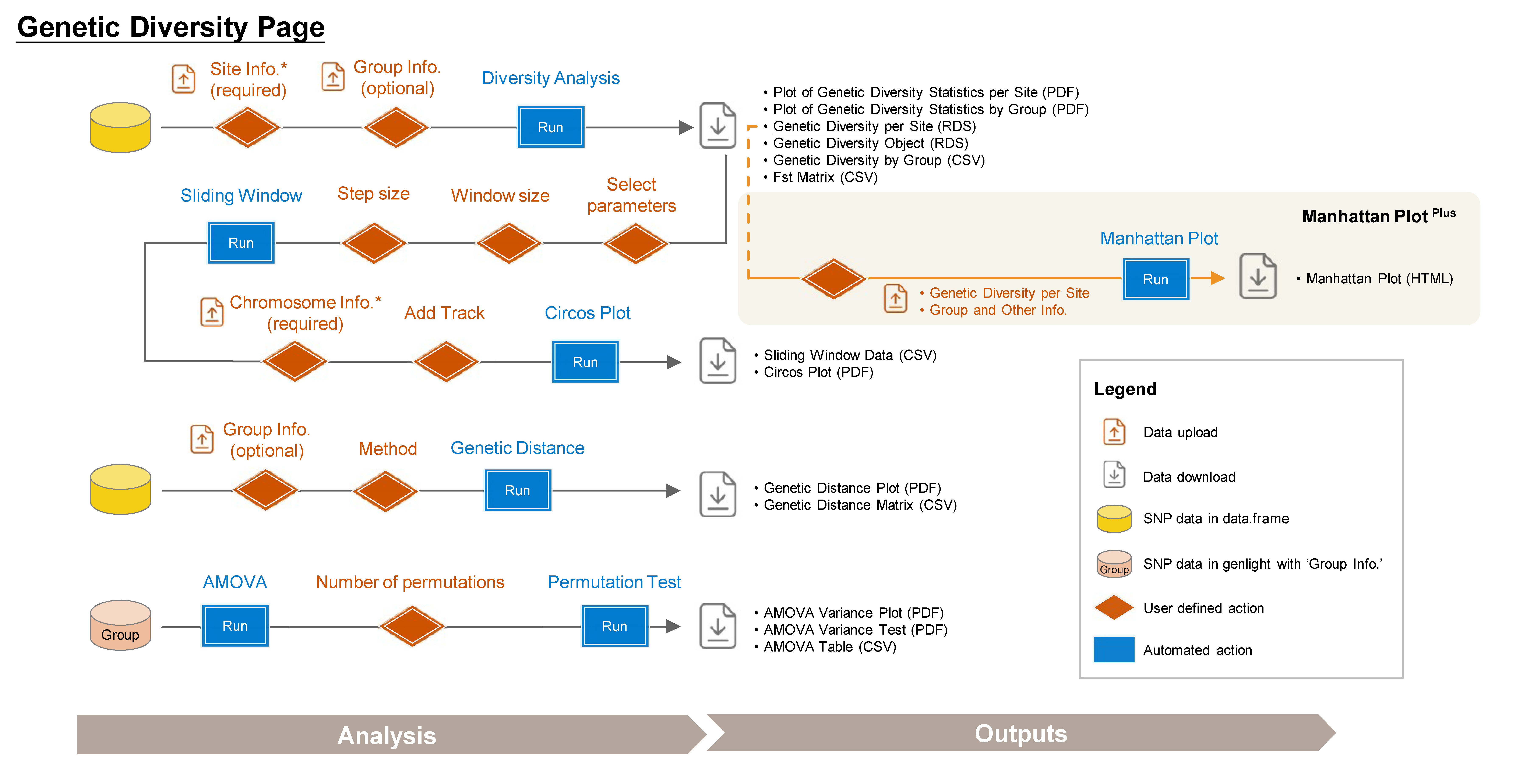
5.1 Diversity Parameter
Calculate key diversity parameters for each SNP site. This approach is performed using the function from snpReady package (Granato et al. 2018).
Required File:
- data.frame
- Site Info. (RDS) of the current data.frame, downloadable from Data Input or Data QC pages.
Note: If you upload Group Info., ensure that each group contains at least 2 samples.
Steps:
Upload Site Info. (required).
-
Upload Group Info. from Population Structure/DAPC subpage (optional). If uploaded, population-based parameters will be calculated.
Click Run Diversity Analysis to generate genetic diversity and the following downloadable files.
Outputs:
- Plot of Genetic Diversity Statistics per Site (PDF): A genome-wide scatter plot visualizing the user-selected parameter.
- Plot of Genetic Diversity Statistics by Group (PDF): A lollipop plot visualizing the user-selected parameter.
- Genetic Diversity per Site (RDS): Contains site information and diversity statistics, can be used as input data in the Selection Sweep/Manhattan PlotPlus.
- Genetic Diversity Object (RDS): Contains all genetic diversity results for future use and reproducibility.
- Genetic Diversity by Group (CSV): A table showing genetic diversity based on defined group assignments.
- Fst Matrix (CSV): A table showing pairwise Fst based on defined group assignments.
5.2 Circos Plot
Genome-wide diversity is visualized using Circos plots generated with the circlize package (Gu et al. 2014) based on results of diversity parameters in a sliding window format.
Required File:
Auto-import the results from the Genetic Diversity/Diversity Parameter subpage.
-
Chromosome Info. (CSV): Reference genome information of the current study.
For more details about this file, refer to Section 2.3 (SNP Density).
Note: Please ensure that each chromosome contains at least one SNP marker.
Step 1: Sliding Window
- Select parameters to generate sliding window data.
- Choose window size (kb) and step size (kp).
- Click Run Sliding Window to generate sliding window data for Circos plot.
Step 2: Circos Plot
- Upload Chromosome Info. (CSV).
- Select a parameter for each track, and add tracks if necessary (up to a maximum of 6).
- Click Run Circos Plot to generate the Circos plot.
Outputs:
- Sliding Window Data (CSV): A sliding window dataset based on user-selected parameters.
- Circos Plot (PDF): This circos plot visualizes the user-selected parameters, highlighting the top 1% of each parameter in red. Chromosome information is displayed on track 1, with coordinates scaled in megabases (Mb).
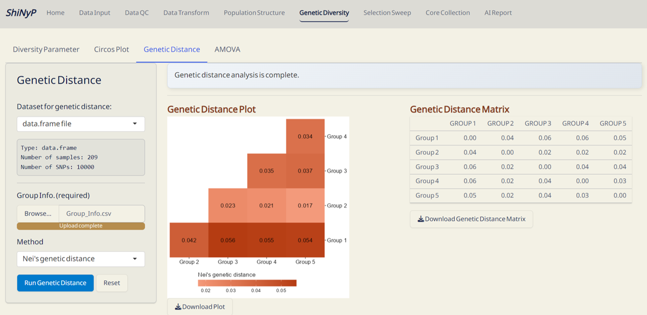
5.3 Genetic Distance
Pairwise genetic distance between populations is computed using hierfstat package. For more information, visit https://rdrr.io/cran/hierfstat/man/genet.dist.html.
5.4 AMOVA (Analysis of MOlecular VAriance)
A method for assessing genetic variations and relationships within and between populations (Excoffier et al. 1992). This approach is performed using the function from hierfstat and poppr packages (Kamvar et al. 2014; GOUDET 2004).
Required File:
- genlight with ‘Group Info.’, downloadable from Data Transform page after you have Group Info.
Step 2: Run Permutation Test
- Choose the number of randomizations for the permutation test to detect the significance of three hierarchical levels. We recommend using 9, 99 (default), 199, 499, 799, or 999 permutations for more classical p-values.
- Click Run Permutation Test to perform the statistical test.
Outputs:
- AMOVA Variance Plot (PDF): A pie chart showing the explained genetic variance of population strata among defined groups.
- AMOVA Variance Test (PDF): A plot showing the significance test of population strata among defined groups. The histograms depict randomized strata distributions, with the black line representing genetic variance components.
- AMOVA Table (CSV): A table with detailed AMOVA results.